10  Reproducible Reporting

10.1 Introduction

Throughout this book, we have been writing R code in separate R scripts. This is great when we are writing code for ourselves. However, this entire book has been centered around reproducibility. An R script can be reproducible, but is limited in how well it communicates results, narrative, and output together in a single place. Sure, you can add comments to help explain what the code is doing, but it does not allow for much text. It also doesn’t show outputs, whether that’s visuals or numbers.

This is exactly where Quarto comes into play. With Quarto, you are able to:

• Write code just as you would in an R script
• Have dedicated spaces for text
• Show outputs for numbers and visuals
• Share with people outside of the R environment

In fact, this entire book was written using Quarto! Each chapter is a different Quarto document all put together. What is fantastic about Quarto is that it is built for the future. It can incorporate code other than R (such as Python), provide you with a better visual preview of your code (see Section 10.4.2), and is a true upgrade from traditional R Markdown.

In this chapter, we are going to go through the benefits of Quarto and how to properly utilize it.

NoteDeeper dive into Quarto

To learn even more about Quarto than this chapter provides, please go to their website: Quarto.

10.2 Learning Objectives

By the end of this chapter, you will be able to:

• Explain the purpose of Quarto and how it supports reproducible research
• Describe the limitations of standalone R scripts for communicating analysis
• Create a new Quarto document and select an appropriate output format
• Identify and modify the core components of a Quarto document, including the YAML, text, and R code chunks
• Write and format narrative text using Markdown syntax
• Create, name, and manage R code chunks to control how code and output are displayed
• Display numerical output, tables, and visualizations within a Quarto document
• Improve table and figure presentation using captions and formatting tools
• Organize analyses using sections and subsections to create a clear document structure
• Render a Quarto document and troubleshoot common rendering errors
• Publish and share Quarto output outside of the R environment
• Apply best practices to ensure a Quarto document is reproducible and understandable on its own

10.3 Creating a Quarto document

When opening a new document, instead of clicking the button for R script, you are going to click the Quarto Document button.

In RStudio: File → New File → Quarto Document.

Once you name it, you have three options to pick from as an output:

1. HTML: Turns your Quarto document into a website
2. PDF: Turns your Quarto document into a PDF
3. Word: Turns your Quarto document into a Microsoft Word document

In this chapter, we will use HTML as our output because it supports interactivity, easy sharing, and web-based reproducibility.

Once you click OK, a brand new Quarto document has been created! If this is your first time looking at a Quarto document, you’re probably thinking, “This looks sort of familiar, but there are some things that are different.” Let’s break down the specific parts of a Quarto document.

10.4 Parts of a Quarto document

Quarto documents are similar to R scripts, but they have more rules and structure. Here, we will be breaking down the different sections.

10.4.1 The YAML

At the top of the document you will find what is called the YAML, which contains the metadata for the document. When you first open a new Quarto Document, it looks like this:

---
title: "Untitled"
format: html
editor: visual
---

It has four default components:

• title: What the title of your Quarto is.
• format: The output you designated the document to be created into
  • There are some cool things you can add here, like change the overall theme or add TOC (table of contents). Like anything in R, take some time to explore and experiment with this.
• editor: tells Quarto (and RStudio) to open the document in the Visual Editor by default, instead of the Source Editor (more about this in Section 10.4.2).

You’ll also notice that the YAML is contained within ---. Besides being at the top of the document, this is Quarto’s way of knowing that this specific part of the document is the YAML.

10.4.2 Source and Visual Panes

In a traditional R script, all of your code is written (for the most part) in the source quadrant (see Section 1.2). If you look towards the top left of the Quarto document, you can see that there are two options adjacent to each other: Source and Visual. Amazingly, Quarto allows you to view what your document looks like in a published format using the Visual pane.

For the most part, anything you can do in one view can be done in the other. Source looks more like an R script, while Visual looks more like a traditional document. I highly suggest playing around and experimenting in both to see the interactivity and capabilities.

There are no wrong answers!

10.4.3 Text

In an R script, every line is dedicated to writing code, with you having to specifically use a # to denote otherwise (as a reminder, in R code, a # comments out whatever is on that line, whether code or text). That is different in Quarto.

Instead of the default being R code, anything you write in a document is treated as text. This is incredibly useful when you want to:

• narrate or tell a story
• describe your code
• describe the output of your code

For instance, what you’re reading right now is text inside a Quarto document. There is no special way of telling Quarto that this content is text, because text is the default.

There are, though, ways to tell Quarto how to format text.

10.4.3.1 Styling Text

Just like in any document, sometimes we want to make particular pieces of text look different. The two most common ways to style text in Quarto are:

Italic: to do this, add * to the beginning and end of your text (whether a single letter, word, sentence, paragraph, etc.).

*It will look like this.*

Bold: to do this, add ** to the beginning and end of your text (whether a single letter, word, sentence, paragraph, etc.).

**It will look like this.**

These are the two basic ways to edit text. What if we need to indent in order to create a list?

10.4.3.2 Adding Lists

As with traditional documents, Quarto is able to create lists, whether that is numbered or bulleted. In order to create a bulleted list, a - and then a space between the text is needed. For a numbered list, you need the number, then a period, then a space before your text. Below are examples of both.

- Text
- More text

1. Text
2. More text

We have seen both of these ample times throughout this textbook, and also in this chapter!

Now that we have talked more about the text portions of a Quarto, let’s now talk about the code portions.

10.4.4 R chunks

Similar to how the YAML used the --- to enclose whatever was inside, for R chunks, Quarto uses “```”. Whatever is inside an R chunk is treated as R code.

Additionally, each R chunk has {}, and inside of that bracket is the letter “r”. This tells Quarto to run the chunk as R code.

It is typically best practice to also name your R chunks. Each one should be a unique name, not only for a way for you to distinguish them from each other, but for R to distinguish them as well. To name your R chunk, you will use the #| (called the hash-pipe) and then the label:.

TipWhat is the #| anyway?

In Quarto, that is used to give information regarding the R chunk, and tells Quarto that anything on this line is not R code to run.

For example, the below code would name an R chunk “r-is-awesome.”

It is best practice to either use one long word or use a - in between your words. In each Quarto document, there are two major types of R chunks.

10.4.4.1 Chunks for R Code

It has already been established that in order to write R code, you need to create an R chunk. Inside an R chunk, you are able to code as normally as you would in an R script. The same rules (even adding comments) apply inside an R chunk. Think of each R chunk as a mini R script.

Take the code below. This, as well as all of the code in the book is written inside R chunks. Below is some code that is from all the way back from section Section 2.4.8 of the book.

library(tidyverse)
library(palmerpenguins)

penguins_new <- penguins %>% 
  select(species, island, bill_length_mm, body_mass_g) %>%
  filter(species == "Adelie") %>%
  mutate(size_category = if_else(body_mass_g >= 3500, "Big","Small")) %>%
  arrange(desc(body_mass_g)) %>% 
  rename(penguin_types = species) 

This code works just as it did in the third chapter. In the Quarto document, all of the code shows. This is an example of how now, for anyone looking, they are able to see your code.

What if we want them to see not only the code, but the output? All we have to do is call what we want to be displayed! For instance, if we want to display the square root of 25 (like in Section 1.3.2):

sqrt(25)

[1] 5

With the above R code, our Quarto document shows both the sqrt(25) code as well as the answer (5).

This is the same no matter if it is square root, ANOVAs, linear regressions, and anything else in this chapter.

TipNaming your R chunks:

Part of making your document reproducible is making sure people can follow along, and part of that is naming your R chunks. To do this, you can use the following: #| label:. The #| lets R know that the information is related to the chunk itself and is not R code, while label: allows you to name the R chunk. You can name it whatever you want, for example:

#| label: first-R-chunk

If your R chunk has a table or graph that will be displayed, you need to tell R that by providing prefixes to your label names. They are as follows:

• tables: tbl-
• figures: fig-

Now let’s move on to displaying tables and graphs.

10.4.4.1.1 Tables

Let’s go back to that penguins_new dataset. Before in section Section C.4.3.2, we “created” it. Now, let’s see what happens when we call the output.

penguins_new

# A tibble: 152 × 5
   penguin_types island    bill_length_mm body_mass_g size_category
   <fct>         <fct>              <dbl>       <int> <chr>        
 1 Adelie        Biscoe              43.2        4775 Big          
 2 Adelie        Biscoe              41          4725 Big          
 3 Adelie        Torgersen           42.9        4700 Big          
 4 Adelie        Torgersen           39.2        4675 Big          
 5 Adelie        Dream               39.8        4650 Big          
 6 Adelie        Dream               39.6        4600 Big          
 7 Adelie        Biscoe              45.6        4600 Big          
 8 Adelie        Torgersen           42.5        4500 Big          
 9 Adelie        Dream               37.5        4475 Big          
10 Adelie        Torgersen           41.8        4450 Big          
# ℹ 142 more rows

By calling penguins_new, the Quarto document now displays the output, which in this case is penguins_new.

TipNaming Table Chunks:

To let Quarto know that there is a table in your R chunk that you are going to display, make sure its name starts with tbl-.

Table 10.1: Showing what a plain table looks like in a Quarto document.

penguins_new

# A tibble: 152 × 5
   penguin_types island    bill_length_mm body_mass_g size_category
   <fct>         <fct>              <dbl>       <int> <chr>        
 1 Adelie        Biscoe              43.2        4775 Big          
 2 Adelie        Biscoe              41          4725 Big          
 3 Adelie        Torgersen           42.9        4700 Big          
 4 Adelie        Torgersen           39.2        4675 Big          
 5 Adelie        Dream               39.8        4650 Big          
 6 Adelie        Dream               39.6        4600 Big          
 7 Adelie        Biscoe              45.6        4600 Big          
 8 Adelie        Torgersen           42.5        4500 Big          
 9 Adelie        Dream               37.5        4475 Big          
10 Adelie        Torgersen           41.8        4450 Big          
# ℹ 142 more rows

Now, that works, but in Quarto, there is an even better way to display tables. Using the knitr package, we can display tables with the kable() function, which is purposely dedicated to displaying tabular data in Quarto.

library(knitr)
kable(head(penguins_new), caption = "This is an example of displaying a table using the kable command. On top of the data looking nicer than just a regular output, we can add a caption (and manipulate other aesthetic pieces.")

Table 10.2: This is an example of displaying a table using the kable command. On top of the data looking nicer than just a regular output, we can add a caption (and manipulate other aesthetic pieces.

penguin_types	island	bill_length_mm	body_mass_g	size_category
Adelie	Biscoe	43.2	4775	Big
Adelie	Biscoe	41.0	4725	Big
Adelie	Torgersen	42.9	4700	Big
Adelie	Torgersen	39.2	4675	Big
Adelie	Dream	39.8	4650	Big
Adelie	Dream	39.6	4600	Big

If we compare and contrast the output from just penguins_new vs the output from the kable() function, there is a stark difference. One of the most important differences is that you can add a caption that can illuminate the table more than just a simple output.

TipCaptions with tables:

You could create a caption for your table using #| tbl-cap: if you were not using kable(). However, it is best practice to use kable().

In the code above, we could have just called penguins_new and not just the head() of penguins_new, so why did we do this?

If we did not call head() then kable() would have produced a table displaying all rows from penguins_new, which would have the user scrolling for a long time. It is always your call as the creator of the document, but keep this in mind:

TipRemember:

You don’t always have to show all your data.

By calling head(), your audience still gets a good picture of what your data looks like.

10.4.4.1.2 Graphs

In Quarto, just how we can display tables, we can also display graphs.

TipNaming Graph Chunks:

To let Quarto know that there is a graph in your R chunk that you are going to display, make sure its name starts with fig-.

Similar to working with tables, when working with graphs and you want to add a caption, you can use fig-cap: on a line with the #|.

library(ggplot2)
ggplot(data = mpg, aes(x = cty, y = hwy)) +
  geom_point()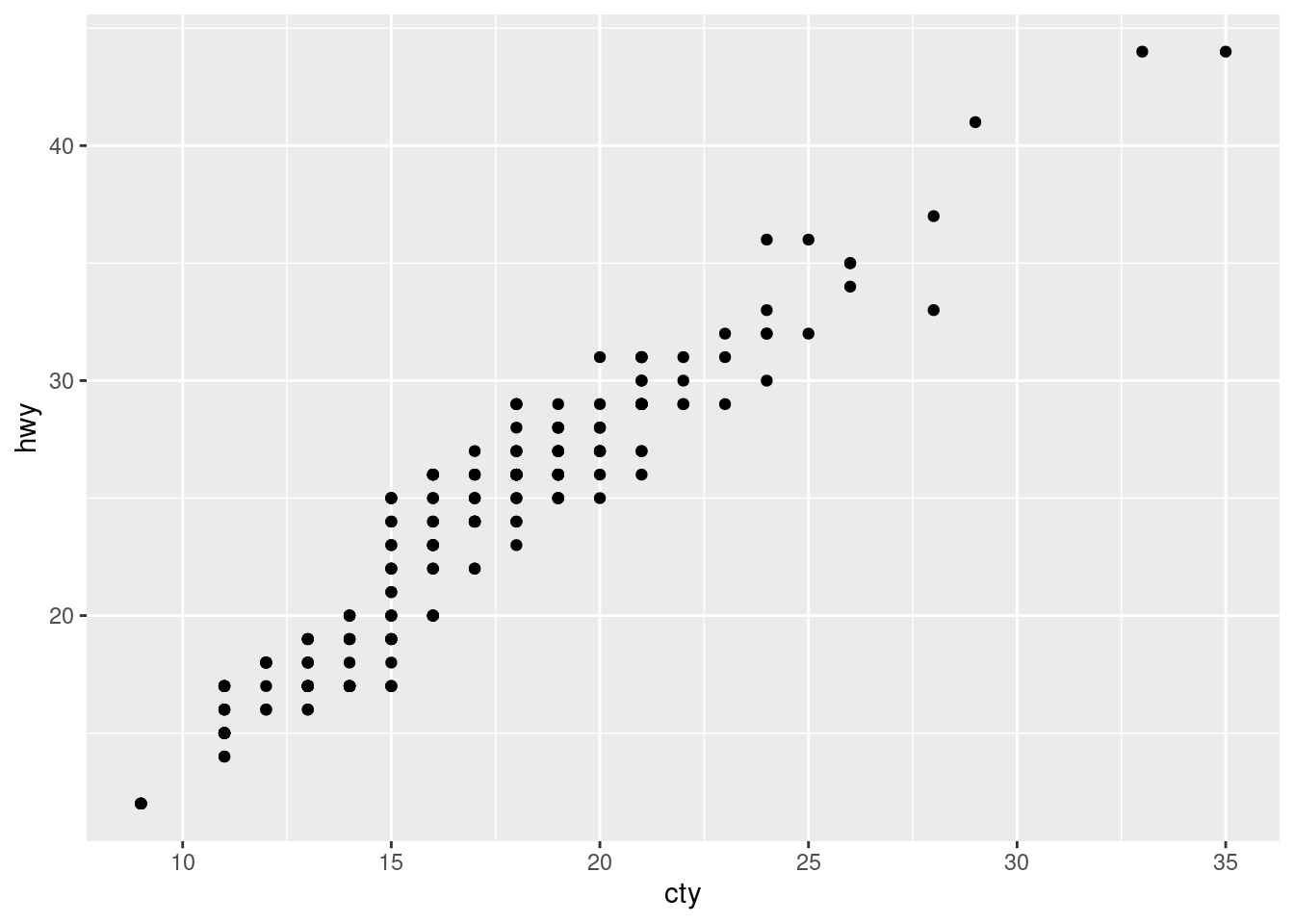

Figure 10.1: An example of a visualization made using ggplot2.

This visualization, which we originally built in Section Section 3.4.2, not only displays the data, but provides a caption to explain the visualization, all thanks to fig-cap:.

Yes, a picture is worth 1,000 words, but sometimes it can be helpful to add some words to help guide viewers.

10.4.5 Sections

One of the most important and powerful parts of a Quarto document is its ability to organize elements into Sections.

Do you see how this chapter, and each chapter of the textbook, are broken down into sections like 10.1, 3.7, etc? Each number represents a different section of the document.

Quarto utilizes the # symbol to set up sections. Here is an example:

# Section 1
# Section 2
## Section 2.1

Notice that a hierarchy is determined through the number of # in the header. Each additional # means one level lower.

Headers, just like R chunks, also need labeling. To do that, inside {} on the same line as the header, add a # within the {} followed up whatever name you want. Just how tables and graphs have specific prefixes, so do section headers, which is sec-. An example of a section name is as follows:

{#sec-creating-sections}

WarningLabel Correctly

Use proper naming convention when naming anything inside your Quarto document.

Lets see why naming is so important in a practical sense.

10.4.6 Cross-Referencing Syntax

I have been emphasizing how important it is to properly name things—whether it is headings, tables, or figures. Naming is vital for organization and reproducibility, but it is also the “secret sauce” for cross-referencing within Quarto documents.

For instance, back in Section 10.4.4.1.2, we created the graph Figure 10.1.

That right there is a cross-reference. By typing @fig-example-ggplot2 in my text, Quarto automatically turned it into a clickable link, with the @ symbol bring the driving factor. It even indexes the figures based on the order they’re created. If I were to add another graph earlier in the chapter, Quarto would automatically update the numbering so this one becomes “Figure 2” without me having to change a thing.

WarningLabeling is Key

This can only be done with proper naming convention, so make sure to properly label your tables and graphs!

10.5 Render a Quarto Document

So far, we have created our Quarto document, filled it with text, code, and we now have something tangible. So, how do we actually see it as an output?

At the top of your screen, you will see a new button that we have not seen before: “Render”. When we press the Render button, we get to see what the finished output looks like. After pressing Render, a pop-up will appear with the outputted version.

WarningIssues with Rendering:

If it does not Render, you will get an error, which will indicate why it failed and what to fix, just like any other error in R.

When your document successfully Renders, you are now ready to proudly share it with your friends, family, colleagues, and the world!

10.6 Publishing a Quarto document

When our document is ready, or “refrigerator-worthy” as I’d call it, we can move a little to the right of the Render button to the “Publish” button. A pop-up will appear with options on where to publish, and Quarto provides their own publishing service Quarto Pub. This is a free hosting website dedicated to sharing R documents (like this).

TipUsing Quarto Pub:

In my family we have a saying:

“If it’s for free, it’s for me!” Quarto Pub is free, and it’s a great place to host your work.

Assuming you do not already have an account, you will sign up for one, input your credentials when prompted, and boom! You will now have your Quarto document online, with a link that you can share with whomever you’d like. With the link, you are now a Quarto author!

10.7 Extras

As stated many times in this book, there are a bevy of things possible in R—and Quarto is no different. Here are a couple of additions you can add to your Quarto document to spice it up.

Mind you, there are more additions you can add to your Quarto document even relating to the sections below. This is just meant to be an introduction.

10.7.1 Links

Like most documents, in Quarto, you are able to add links for your viewers to be directed to. This was actually done in the introduction to R chapter with the link to all of the CRAN packages. The formula for adding a link is this

1. []: What you want the link you click on to be displayed as.
2. (): The link you want viewers to be directed to.

This is what the code looks like:

[here](https://r-packages.io/packages).

What is inside the brackets is what the viewers see, and then what is inside the parentheses is the link they’ll be directed to if they click on the link.

10.7.2 Pictures

In chapter 3, I showed you all a picture of an Adelie penguin. Below is the code I used to display the image:

![A picture of an Adelie penguin.](Adelie-Screenshot.png)

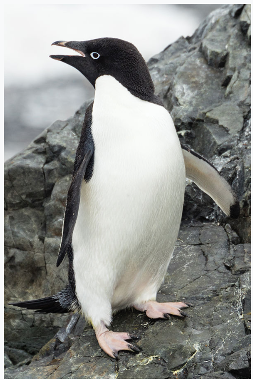The formula for this goes:

• !: Letting R know that you’re about to add a picture.
• []: Providing a description for the picture for people unable to see the picture.
• (): The link to the picture.
  • The image needs to live in the same part of your computer that your Quarto document lives.

10.7.3 Checklists

In most of the chapters in the textbook, a checklist at the end is provided. This is to help you along your analyses to make sure you’re hitting all of the major components of the analysis.

To create a checklist, is it quite similar to how to create lists. Below is an example:

- [ ] Identified both variables as **categorical** (not numeric)?

There is still a -, followed by a space. However, after the space is [] with a space separating the two brackets. This space is so you can click inside the checkbox.

10.7.4 Standout Sections

There are times where you may want specific text to stand out. In this book, an example (and my favorite), stemming all the way from chapter 1, is:

R puts the r in Artist.

To do this, all you need is the > on its own line. The code looks like this:

> R puts the r in Artist.

Simple as that! This can be a vital addition when used correctly.

10.7.5 Callout Boxes

Throughout this book, there have been many callout boxes. These typically have been with tips, notes, and sometimes even warnings. Here is an example of the first ever one found back in chapter 1:

TipData is art, and as you will read many times in this book:

R puts the r in Artist.

Below is the code on how to create them. It starts with ::: and ends with :::,

::: {.callout-tip}
## Data is art, and as you will read many times in this book:
R puts the **r** in Artist.
:::

There are a few things to notice:

• The callout boxes start and end with :::.
• {callout-}: This tells R that it is all callout box, and whatever is after the - tell it which type of callout box it is. The choices are:
  • tip
  • note
  • warning
  • important
  • caution
• Anything after the {callout-} is text inside the box.

These can be a fantastic tool to help guide your readers through whatever analytical, reproducible story you’re trying to tell in your Quarto documents.

10.7.6 Changing Settings for Specific R Chunks

To the right of each R chunk there is a circular gear icon. Here is where you can change some of the settings of each R chunk. There are three things you’ll see:

1. Chunk Name: This is where you can also name your chunk.
2. Output: This is where you can control the output of the specific R chunk. It is by default set to the document default, but this can be altered for individual R chunks.
3. Slider options: You can further customize the output of an individual R chunk with these four options. You’ll mostly be interested in the first two, as they’re typically the most powerful. For instance, when you first load tidyverse a big message appears, which you can stop by switching “Show messages” to the left.

ImportantThe gear icon and the #|

You will notice that each of these manipulations add a line to the beginning of the R chunk, each starting the #|.

Each R chunk is unique and requires different settings based on what is inside and what you want the viewer to see from it.

10.8 Key Takeaways

• Quarto allows you to combine code, narrative text, and output in a single document, making analyses easier to understand, evaluate, share, and reproduce.
• While a standalone R script can be reproducible, Quarto strengthens reproducibility by explicitly linking analytical decisions, results, and interpretation in one place.
• Every Quarto document is built around three core components: YAML metadata, Markdown text, and R code chunks.
• The YAML section controls document-level settings such as the title, author, date, output format, and optional features like themes and tables of contents.
• Narrative text in Quarto is written using Markdown syntax, allowing you to structure and format reports without writing additional code.
• All R code must be written inside R chunks, which are executed from top to bottom each time the document is rendered.
• Naming R chunks clearly helps organize analyses, improves readability, and prevents rendering errors.
• Any object, function, table, or plot that is called inside a chunk will automatically appear in the final output.
• Tables and figures can be enhanced with captions and formatting to make results easier to interpret and reference.
• Cross-referencing automates the connection between your narrative and your results; by using the @ symbol with proper prefixes (fig-, tbl-, or sec-), Quarto handles all numbering and hyperlinking for you, ensuring your document remains organized even as you add or move content.
• Rendering a Quarto document runs the entire analysis in a clean session, helping expose missing packages, undefined objects, and hidden dependencies.
• Publishing a Quarto document transforms an analysis into a polished, shareable artifact that can be viewed outside of R.
• This chapter demonstrates how all earlier analytical skills—data wrangling, visualization, and modeling—come together in a clear, reproducible final report.

10.9 Checklist

When creating a Quarto document, have you:

• Selected an appropriate output format (HTML, PDF, or Word) based on how the document will be shared?
• Clearly defined document metadata in the YAML (title, author, date, output)?
• Written narrative text that explains why analytical decisions were made, not just what the code does?
• Organized the document into logical sections using headers (#, ##, ###)?
• Named your R chunks clearly so their purpose is easy to understand?
• Loaded all required packages within the document to ensure reproducibility?
• Confirmed that the document renders successfully from top to bottom without errors?
• Checked that all tables and figures are readable and appropriately formatted?
• Added informative captions to tables (tbl-cap) and figures (fig-cap) where explanation is helpful?
• Utilized cross-references (@) for sections, tables, and figures to help the reader navigate the document?
• Avoided displaying unnecessary or distracting output (e.g., very large tables or intermediate objects)?
• Used text formatting (bold, italics, lists, quotes) intentionally to guide the reader?
• Asked yourself: Could someone unfamiliar with this project understand the analysis by reading this document alone?

10.10 Key Functions & Commands

The following functions and commands are introduced or reinforced in this chapter to support reproducible reporting and polished output in Quarto documents.

• R code chunks
  • Encapsulate all executable R code and ensure analyses run in a controlled, reproducible order.
• Chunk metadata (#|)
  • Used to label chunks, control output behavior, and add captions for tables and figures.
• kable() (knitr)
  • A convenient tool for displaying clean, readable tables in rendered Quarto output.
• Rendering
  • Executes the entire document in a fresh session, producing a complete, reproducible report.

10.11 Summary of Common Quarto Syntax

In addition to R functions, Quarto relies on a small set of Markdown syntax rules to format text and structure documents. These elements are not functions, but they are essential for writing clear, readable, and professional reports.

• Text emphasis:
  • *text*: Italicizes text.
  • **text**: Bolds text.
  • ***text***: Bold and italic text.
• Headings:
  • #: Primary heading (chapter-level).
  • ##: Section heading.
  • ###: Subsection heading.
  • {#sec-name}: Added after a header to create a label for cross-referencing.
• Lists:
  • -: Creates a bulleted list.
  • 1.: Creates a numbered list.
  • [ ]: Creates a checklist.
• Links:
  • [text](url): Creates a clickable hyperlink.
• Images:
  • ![alt text](path): Inserts an image into the document, with alternative text for accessibility.
• Block quotes:
  • >: Highlights a block of text, often used for emphasis or reflection.
• Callout boxes
  • ::: {.callout-tip}: Highlights helpful tips or best practices.
  • ::: {.callout-note}: Provides additional context or clarification.
  • ::: {.callout-warning}: Draws attention to potential problems or common mistakes.
  • ::: {.callout-important}: Emphasizes critical information that should not be overlooked.
  • ::: {.callout-caution}: Signals situations that require extra care.
  • :::: Ends a callout box.
• Cross-Referencing
  • @: The symbol used to trigger a link to a label (e.g., @sec-name, @fig-name, or @tbl-name).

10.12 Common Rendering Errors and How to Fix Them

• Object not found: An object is used before it is created.
  • Fix: Make sure all objects are defined earlier in the document and not only in the R environment.
• Missing package: A required package is not loaded or installed.
  • Fix: Load all necessary packages inside the Quarto document using library().
• Duplicate chunk labels: Two R chunks share the same name.
  • Fix: Ensure every R chunk has a unique #| label:.
• File not found: An image or data file cannot be located.
  • Fix: Check file names, capitalization, and that files are stored in the correct directory.
• Code runs in console but not when rendering: The document relies on objects outside the file.
  • Fix: Restart R and render the document to confirm it runs in a clean session.

10.13 💡 Reproducibility Tip:

A reproducible Quarto document should render successfully from top to bottom in a clean R session without manual fixes.

Because rendering re-runs every chunk in order, it helps expose missing packages, undefined objects, and hidden dependencies that can make analyses difficult to reproduce. To support this, always load required packages within the document and avoid relying on objects created outside the document.

TipMaking sure your Quarto document runs in any R Session:

You can check whether these criteria are met by shutting down your R session completely, opening your Quarto document in a brand new R session, and pressing Render.

An analysis is only reproducible if it can be re-run and understood as a complete, self-contained document.