install.packages("tidyverse")2 Introduction To tidyverse
Just like Spider-Man, we are going to enter a new universe in R: the tidyverse!
This chapter introduces the tidyverse, a collection of R packages designed to make data analysis more readable, consistent, and reproducible. The tools introduced here will be used repeatedly throughout the remainder of this textbook, forming the backbone of nearly every analysis we perform.
As discussed in the last chapter, R comes with prebuilt functions, but what makes R so dynamic and powerful is the ability to install and use different libraries. Few have been as impactful or as widely used as the tidyverse package. Now, of course, you can use R however you would like, as your programming style is totally up to you. The tidyverse, however, has been unofficially accepted as the major dialect of R.
2.1 Learning Objectives
By the end of this chapter, you will be able to:
- Install and load R packages from CRAN
- Explain what the tidyverse is and why it is commonly used
- Use the pipe operator (
%>%) to build readable data workflows - Select, filter, arrange, and rename variables in a data frame
- Create new variables using
mutate() - Apply conditional logic with
if_else()andcase_when() - Summarize grouped data using
group_by()andsummarize() - Combine multiple tidyverse verbs into a single reproducible pipeline
Before we get started, we have to first install tidyverse.
2.2 Using Packages
The Comprehensive R Archive Network (CRAN) is where all of the packages are hosted in R, and when installing packages, this is where they will be installed from.
We briefly spoke about packages in Section 1.8, but now let’s take a deeper dive.
2.2.1 Installing Packages
In order to install packages, we can utilize the install.packages() command. Let’s install our first official package, the tidyverse package.
Awesome! It may take a second or two for the code to run, but tidyverse has now been installed in R. Importantly, once a package is installed on your local computer, you don’t need to install it again. To get a little more practice, let’s install some more packages that we will be using.
install.packages("palmerpenguins")
install.packages("fortunes")
install.packages("cowsay")
2.2.2 Loading Packages
As stated before, once a package has been installed, it does not need to be reinstalled every time you utilize R. However, each time you want to use a package in an R session, you do need to load it. This can be done using the command library().
library(tidyverse)Warning: package 'readr' was built under R version 4.5.2Warning: package 'purrr' was built under R version 4.5.2── Attaching core tidyverse packages ──────────────────────── tidyverse 2.0.0 ──
✔ dplyr 1.1.4 ✔ readr 2.1.5
✔ forcats 1.0.1 ✔ stringr 1.6.0
✔ ggplot2 4.0.0 ✔ tibble 3.3.0
✔ lubridate 1.9.4 ✔ tidyr 1.3.1
✔ purrr 1.2.0
── Conflicts ────────────────────────────────────────── tidyverse_conflicts() ──
✖ dplyr::filter() masks stats::filter()
✖ dplyr::lag() masks stats::lag()
ℹ Use the conflicted package (<http://conflicted.r-lib.org/>) to force all conflicts to become errorslibrary(palmerpenguins)Warning: package 'palmerpenguins' was built under R version 4.5.2
Attaching package: 'palmerpenguins'

The following objects are masked from 'package:datasets':

penguins, penguins_rawlibrary(fortunes)
library(cowsay)
# Quick sanity check that packages are loaded
sessionInfo()$otherPkgs %>% names() [1] "cowsay" "fortunes" "palmerpenguins" "lubridate"
[5] "forcats" "stringr" "dplyr" "purrr"
[9] "readr" "tidyr" "tibble" "ggplot2"
[13] "tidyverse" We have successfully loaded all of the packages (and in turn all of their contents). That means that as long as we do not close this R session, we can utilize the packages.
The palmerpenguins package we will be using in this chapter. Before then, I want to show you that R is fun and diverse. The package fortunes provides you a random R quote with the function fortune() and the say() command from the cowsay package provides a beautiful animal saying whatever you want it to say. Below the animal is “cow” but try some other ones (I suggest “dragon”).
# Fun packages
fortunes::fortune()   # random quote about R
Roger D. Peng: I don't think anyone actually believes that R is designed to
make *everyone* happy. For me, R does about 99% of the things I need to do, but
sadly, when I need to order a pizza, I still have to pick up the telephone.
Douglas Bates: There are several chains of pizzerias in the U.S. that provide
for Internet-based ordering (e.g. www.papajohnsonline.com) so, with the
Internet modules in R, it's only a matter of time before you will have a
pizza-ordering function available.
Brian D. Ripley: Indeed, the GraphApp toolkit (used for the RGui interface
under R for Windows, but Guido forgot to include it) provides one (for use in
Sydney, Australia, we presume as that is where the GraphApp author hails from).
Alternatively, a Padovian has no need of ordering pizzas with both home and
neighbourhood restaurants ....
   -- Roger D. Peng, Douglas Bates, and Brian D. Ripley
R-help (June 2004)cowsay::say("Welcome to tidyverse!", by = "cow")
 _______________________
< Welcome to tidyverse! >
 -----------------------
      \
       \

        ^__^
        (oo)\ ________
        (__)\         )\ /\
             ||------w|
             ||      ||
It isn’t always necessary, nor will it be done a lot in this book, but you can use the :: before the command to specifically mention what package the command is coming from. Most of the time this isn’t necessary, but there are times when you will have packages loaded that have overlapping function names. This is when :: should be called.
To further illustrate the diversity of R packages, let’s introduce an example of working with live, real-world data using the nycOpenData package. This package connects directly to the NYC Open Data Portal and displays the most recent data happening in the city. By using the nyc_311() function, we can gather the five most recent 311 calls in New York City. The fun thing is that every time you open this chapter, this data will be different! This is an important aspect of working with live data and needs to be considered when creating reproducible research.
First we install the package.
install.packages("nycOpenData")Now we load it and call the function.
library(nycOpenData)
head(nyc_311())
# A tibble: 6 × 45
unique_key created_date agency agency_name complaint_type descriptor
<chr> <chr> <chr> <chr> <chr> <chr>
1 67572042 2026-01-23T02:20:59.0… NYPD New York C… Noise - Resid… Loud Musi…
2 67573444 2026-01-23T02:20:43.0… NYPD New York C… Noise - Resid… Banging/P…
3 67573446 2026-01-23T02:19:18.0… NYPD New York C… Noise - Resid… Loud Musi…
4 67572026 2026-01-23T02:18:00.0… NYPD New York C… Illegal Parki… Commercia…
5 67572056 2026-01-23T02:17:52.0… NYPD New York C… Non-Emergency… Trespassi…
6 67572044 2026-01-23T02:17:44.0… NYPD New York C… Noise - Resid… Loud Musi…
# ℹ 39 more variables: location_type <chr>, incident_zip <chr>,
# incident_address <chr>, street_name <chr>, cross_street_1 <chr>,
# cross_street_2 <chr>, intersection_street_1 <chr>,
# intersection_street_2 <chr>, address_type <chr>, city <chr>,
# landmark <chr>, status <chr>, community_board <chr>,
# council_district <chr>, police_precinct <chr>, bbl <chr>, borough <chr>,
# x_coordinate_state_plane <chr>, y_coordinate_state_plane <chr>, …With some examples under our belt, let’s move to the tidyverse!
2.3 Meet the tidyverse
Last chapter, R was introduced. In this chapter, we will be building on the basic language and syntax we learned and build upon it with tidyverse.
2.3.1 The Pipe
One of the best things that the tidyverse has to offer is called piping. It technically comes from the magrittr package. What makes the tidyverse package so ubiquitous with R is that tidyverse is actually a collection of R packages in one package. By installing and loading the tidyverse package, you are actually installing and loading a bevy of packages and significantly powering up your R session. Here are the packages included in tidyverse:
dplyr- Tools for data manipulation, including
select(),filter(),mutate(),arrange(), andsummarize().
- Tools for data manipulation, including
ggplot2- A powerful system for creating data visualizations using the grammar of graphics.
tidyr- Tools for reshaping and cleaning data, such as
pivot_longer()andpivot_wider().
- Tools for reshaping and cleaning data, such as
readr- Functions for reading data into R (e.g., CSV files) quickly and consistently.
tibble- A modern reimagining of data frames with improved printing and behavior.
stringr- Tools for working with text data, such as
str_trim()andstr_to_upper().
- Tools for working with text data, such as
forcats- Tools for working with categorical (factor) variables.
Piping is telling R the sequence you want things to be done in code, and uses %>%. Below is an example of how you would write something.
# In base R, to find the square root of a number, we would use this:
sqrt(42)
[1] 6.480741# With piping, we could rewrite it like this:
42 %>% sqrt()[1] 6.480741In base R, code is written inside out. What I mean by that is that base R code is often evaluated from the inside out. You take the 42 (inside the square root) and then square root it. With piping, it is read left to right. First this, then this, etc.
Let’s use a more potent example. You’re starting this book and have been thinking, ” i love r! “. It is all lowercase and has whitespace before and after the words. However, you love R so much you want it to be in all caps, and you don’t want whitespace ruining your exclamation. Below is the way to do this in base R and then using piping.
For reference, the str_to_upper() command capitalizes everything in a string, and the str_trim() removes leading and trailing whitespace in a string. Both are a part of the stringr package in the tidyverse.
str_to_upper(str_trim(" i love r! "))[1] "I LOVE R!"" i love r! " %>% str_trim() %>% str_to_upper()[1] "I LOVE R!"# You can also move down instead if you like
# " Adelie " %>%
# str_trim() %>%
# str_to_upper()Those two pieces of code do the same thing, but they look very different:
- The first reads right to left, or middle to outer. It starts with the string inside the
str_trim(), then you have to move outward to thestr_to_upper(), moving right to left moving from parenthesis to parenthesis. - The second reads left to right. It goes string %>% function %>% function. It takes the string, trims the whitespace, then turns it to uppercase.
The first starts with a function, the second starts with what we want the function(s) to be applied to.
TipWhen piping, the rule of thumb is:
Each line in a pipeline should perform one clear transformation.
2.4 Manipulating Data in tidyverse
We will now be utilizing another one of our packages that we installed and loaded, the palmerpenguins package. It has the dataset penguins that we are going to use. If you use the helper function and write ?palmerpenguins or ?penguins you will find a description of the data (hint: it’s data related to penguins).
Each of the subsections touches on a different aspect. Let’s start by finding out more about our data.
2.4.1 Distinct
We have a dataset that we don’t quite know too much about. Let’s first find out some information about it using what we learned from base R in the last chapter.
ncol(penguins) # Finding out the number of columns[1] 8nrow(penguins) # Finding out the number of rows[1] 344colnames(penguins) # Finding out the names of the columns[1] "species" "island" "bill_length_mm"
[4] "bill_depth_mm" "flipper_length_mm" "body_mass_g"
[7] "sex" "year" Great, we now know that there are 344 rows of data, 8 columns, and all the column names. We know that there are different types of penguins, and that the species is a column in this dataset. We could scroll through every single row and try to eyeball the distinct types of penguin species in this dataset. Or we could use the distinct() function to get this information.
Tip
distinct()
Keep only distinct rows from a data frame.
penguins %>% distinct(species)# A tibble: 3 × 1
species
<fct>
1 Adelie
2 Gentoo
3 ChinstrapThat one line of code filtered through all 344 rows and figured out that there are only three different species of penguins in the penguins dataset. But it doesn’t stop there - you can also use the distinct() command to see distinct combinations of data too. For example:
penguins %>% distinct(species, island)# A tibble: 5 × 2
species island
<fct> <fct>
1 Adelie Torgersen
2 Adelie Biscoe
3 Adelie Dream
4 Gentoo Biscoe
5 Chinstrap Dream Very interesting! We can see that the “Adelie” species is found on three different islands, whereas the other two species are only found on one island each (and different islands). With just a comma, you can find the distinct combinations between data in any of your columns.
Now, what if we don’t need all of our columns?
2.4.2 Select
For now, let’s pretend like we only want to work with the columns species, island, bill_length_mm, and body_mass_g. How do we select for only those? We can use the select() command!
Tip
select()
Changes which columns exist.
penguins %>% select(species, island, bill_length_mm, body_mass_g)# A tibble: 344 × 4
species island bill_length_mm body_mass_g
<fct> <fct> <dbl> <int>
1 Adelie Torgersen 39.1 3750
2 Adelie Torgersen 39.5 3800
3 Adelie Torgersen 40.3 3250
4 Adelie Torgersen NA NA
5 Adelie Torgersen 36.7 3450
6 Adelie Torgersen 39.3 3650
7 Adelie Torgersen 38.9 3625
8 Adelie Torgersen 39.2 4675
9 Adelie Torgersen 34.1 3475
10 Adelie Torgersen 42 4250
# ℹ 334 more rowsInstead of using the actual column names, we can use the column indices - which number (in order). Below is an example using the column indexes (hint: it uses a comma and a colon.)
# This is saying let's take the first column, and then every column from 3 to 5
penguins %>% select(1,3:5)
# A tibble: 344 × 4
species bill_length_mm bill_depth_mm flipper_length_mm
<fct> <dbl> <dbl> <int>
1 Adelie 39.1 18.7 181
2 Adelie 39.5 17.4 186
3 Adelie 40.3 18 195
4 Adelie NA NA NA
5 Adelie 36.7 19.3 193
6 Adelie 39.3 20.6 190
7 Adelie 38.9 17.8 181
8 Adelie 39.2 19.6 195
9 Adelie 34.1 18.1 193
10 Adelie 42 20.2 190
# ℹ 334 more rowsNote that no matter if we specifically named the columns or used their index numbers, we get the same result. However using column numbers works, but can break if the dataset changes.
Now that we can select what columns we want to see, it is time to filter what rows we want. Below are some of the operators we are going to use to filter our data.
==: Equal to!=: Not equal to>=: Greater than or equal to<=: Less than or equal to>: Greater than<: Less than&: And|: Or%in%: Within
2.4.3 Filter
When we want to select for specific columns in a dataset, we use the select() command. But, when we want to filter the data inside a dataset, we utilize the filter() command.
Tip
filter()
Changes which rows exist.
Let’s say that we want to filter for only the penguin species Adelie. If you do not know what they look like, here is a picture:
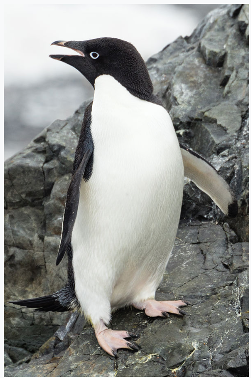
We will filter for only rows that have the word Adelie inside the species column.
penguins %>%
  filter(species == "Adelie")
# A tibble: 152 × 8
species island bill_length_mm bill_depth_mm flipper_length_mm body_mass_g
<fct> <fct> <dbl> <dbl> <int> <int>
1 Adelie Torgersen 39.1 18.7 181 3750
2 Adelie Torgersen 39.5 17.4 186 3800
3 Adelie Torgersen 40.3 18 195 3250
4 Adelie Torgersen NA NA NA NA
5 Adelie Torgersen 36.7 19.3 193 3450
6 Adelie Torgersen 39.3 20.6 190 3650
7 Adelie Torgersen 38.9 17.8 181 3625
8 Adelie Torgersen 39.2 19.6 195 4675
9 Adelie Torgersen 34.1 18.1 193 3475
10 Adelie Torgersen 42 20.2 190 4250
# ℹ 142 more rows
# ℹ 2 more variables: sex <fct>, year <int>With that piece of code, the output only returned rows where Adelie is the species.
Thankfully, we do not have to keep to only one filter condition at a time.
2.4.3.1 Filtering with AND/OR
Inside the same filter() command, we can have as many conditions as possible. One incredibly important decision is whether to use and/or.
In the case we only want to return rows where species is “Adelie” and the island is “Torgersen”, we will use the & symbol.
Important: rows that return have to meet both criteria. If in that row either none, or even one, of the criteria are met, then that row will not return.
penguins %>%
  filter(species == "Adelie" & island == "Torgersen")
# A tibble: 52 × 8
species island bill_length_mm bill_depth_mm flipper_length_mm body_mass_g
<fct> <fct> <dbl> <dbl> <int> <int>
1 Adelie Torgersen 39.1 18.7 181 3750
2 Adelie Torgersen 39.5 17.4 186 3800
3 Adelie Torgersen 40.3 18 195 3250
4 Adelie Torgersen NA NA NA NA
5 Adelie Torgersen 36.7 19.3 193 3450
6 Adelie Torgersen 39.3 20.6 190 3650
7 Adelie Torgersen 38.9 17.8 181 3625
8 Adelie Torgersen 39.2 19.6 195 4675
9 Adelie Torgersen 34.1 18.1 193 3475
10 Adelie Torgersen 42 20.2 190 4250
# ℹ 42 more rows
# ℹ 2 more variables: sex <fct>, year <int>That returned exactly what we wanted. But, what if we changed our mind. We want to return rows that either have “Adelie” as their species or the island is “Torgersen”. Instead of using the & symbol, we need to use the | symbol.
penguins %>%
  filter(species == "Adelie" | island == "Torgersen")
# A tibble: 152 × 8
species island bill_length_mm bill_depth_mm flipper_length_mm body_mass_g
<fct> <fct> <dbl> <dbl> <int> <int>
1 Adelie Torgersen 39.1 18.7 181 3750
2 Adelie Torgersen 39.5 17.4 186 3800
3 Adelie Torgersen 40.3 18 195 3250
4 Adelie Torgersen NA NA NA NA
5 Adelie Torgersen 36.7 19.3 193 3450
6 Adelie Torgersen 39.3 20.6 190 3650
7 Adelie Torgersen 38.9 17.8 181 3625
8 Adelie Torgersen 39.2 19.6 195 4675
9 Adelie Torgersen 34.1 18.1 193 3475
10 Adelie Torgersen 42 20.2 190 4250
# ℹ 142 more rows
# ℹ 2 more variables: sex <fct>, year <int>Now, instead of returning rows that have both “Adelie” and “Torgersen”, the code returns rows where either species is equal to “Adelie” or island is equal to “Torgersen.”
2.4.3.2 Logical Filters
We do not have to just use ==, as we have other options. Below are two options: the first filters for any body mass over 4,000 grams, and the second filters for species that are either Adelie or Gentoo.
penguins %>% filter(body_mass_g >= 4000)# A tibble: 177 × 8
species island bill_length_mm bill_depth_mm flipper_length_mm body_mass_g
<fct> <fct> <dbl> <dbl> <int> <int>
1 Adelie Torgersen 39.2 19.6 195 4675
2 Adelie Torgersen 42 20.2 190 4250
3 Adelie Torgersen 34.6 21.1 198 4400
4 Adelie Torgersen 42.5 20.7 197 4500
5 Adelie Torgersen 46 21.5 194 4200
6 Adelie Dream 39.2 21.1 196 4150
7 Adelie Dream 39.8 19.1 184 4650
8 Adelie Dream 44.1 19.7 196 4400
9 Adelie Dream 39.6 18.8 190 4600
10 Adelie Dream 42.3 21.2 191 4150
# ℹ 167 more rows
# ℹ 2 more variables: sex <fct>, year <int>penguins %>% filter(species %in% c("Adelie", "Gentoo"))# A tibble: 276 × 8
species island bill_length_mm bill_depth_mm flipper_length_mm body_mass_g
<fct> <fct> <dbl> <dbl> <int> <int>
1 Adelie Torgersen 39.1 18.7 181 3750
2 Adelie Torgersen 39.5 17.4 186 3800
3 Adelie Torgersen 40.3 18 195 3250
4 Adelie Torgersen NA NA NA NA
5 Adelie Torgersen 36.7 19.3 193 3450
6 Adelie Torgersen 39.3 20.6 190 3650
7 Adelie Torgersen 38.9 17.8 181 3625
8 Adelie Torgersen 39.2 19.6 195 4675
9 Adelie Torgersen 34.1 18.1 193 3475
10 Adelie Torgersen 42 20.2 190 4250
# ℹ 266 more rows
# ℹ 2 more variables: sex <fct>, year <int>2.4.3.3 Filtering NA values
In any dataset, NA values can be a pain. Depending what to do with them is always situational, but it is important to learn how to work with them. We can utilize is.na() to filter for which are NA and the drop_na() to remove all rows that have at least one NA value.
penguins %>% filter(is.na(body_mass_g)) # Filter for rows that have missing data# A tibble: 2 × 8
species island bill_length_mm bill_depth_mm flipper_length_mm body_mass_g
<fct> <fct> <dbl> <dbl> <int> <int>
1 Adelie Torgersen NA NA NA NA
2 Gentoo Biscoe NA NA NA NA
# ℹ 2 more variables: sex <fct>, year <int>penguins %>% drop_na(body_mass_g) # Filters for rows that don't have missing data# A tibble: 342 × 8
species island bill_length_mm bill_depth_mm flipper_length_mm body_mass_g
<fct> <fct> <dbl> <dbl> <int> <int>
1 Adelie Torgersen 39.1 18.7 181 3750
2 Adelie Torgersen 39.5 17.4 186 3800
3 Adelie Torgersen 40.3 18 195 3250
4 Adelie Torgersen 36.7 19.3 193 3450
5 Adelie Torgersen 39.3 20.6 190 3650
6 Adelie Torgersen 38.9 17.8 181 3625
7 Adelie Torgersen 39.2 19.6 195 4675
8 Adelie Torgersen 34.1 18.1 193 3475
9 Adelie Torgersen 42 20.2 190 4250
10 Adelie Torgersen 37.8 17.1 186 3300
# ℹ 332 more rows
# ℹ 2 more variables: sex <fct>, year <int>As a cautionary tale, always be careful with how you handle NA values, as different situations really do require different handling of NA values.
Now, we will move on to how we want our data to be organized.
2.4.4 Arrange
Organization of data is just as important as anything else. Most likely, data is not prearranged in any particular order. Luckily, the arrange() command allows us to organize our data very nicely. There are only two options: ascending or descending order. By default, arrange() orders the data in ascending order.
Tip
arrange()
orders the rows of a data frame.
penguins %>% arrange(body_mass_g) # ascending order# A tibble: 344 × 8
species island bill_length_mm bill_depth_mm flipper_length_mm body_mass_g
<fct> <fct> <dbl> <dbl> <int> <int>
1 Chinstrap Dream 46.9 16.6 192 2700
2 Adelie Biscoe 36.5 16.6 181 2850
3 Adelie Biscoe 36.4 17.1 184 2850
4 Adelie Biscoe 34.5 18.1 187 2900
5 Adelie Dream 33.1 16.1 178 2900
6 Adelie Torgers… 38.6 17 188 2900
7 Chinstrap Dream 43.2 16.6 187 2900
8 Adelie Biscoe 37.9 18.6 193 2925
9 Adelie Dream 37.5 18.9 179 2975
10 Adelie Dream 37 16.9 185 3000
# ℹ 334 more rows
# ℹ 2 more variables: sex <fct>, year <int>penguins %>% arrange(desc(body_mass_g)) # descending order# A tibble: 344 × 8
species island bill_length_mm bill_depth_mm flipper_length_mm body_mass_g
<fct> <fct> <dbl> <dbl> <int> <int>
1 Gentoo Biscoe 49.2 15.2 221 6300
2 Gentoo Biscoe 59.6 17 230 6050
3 Gentoo Biscoe 51.1 16.3 220 6000
4 Gentoo Biscoe 48.8 16.2 222 6000
5 Gentoo Biscoe 45.2 16.4 223 5950
6 Gentoo Biscoe 49.8 15.9 229 5950
7 Gentoo Biscoe 48.4 14.6 213 5850
8 Gentoo Biscoe 49.3 15.7 217 5850
9 Gentoo Biscoe 55.1 16 230 5850
10 Gentoo Biscoe 49.5 16.2 229 5800
# ℹ 334 more rows
# ℹ 2 more variables: sex <fct>, year <int>2.4.5 Mutate
Last chapter, we learned that in order to create a new column, we could do so using the $ symbol. In tidyverse, we can also create new columns, but instead of using the $, we can use the mutate() command.
Tip
mutate()
Changes or creates columns.
# Base R
penguins$bill_ratio <- penguins$bill_length_mm / penguins$bill_depth_mm

penguins<- penguins %>%
  mutate(bill_ratio = bill_length_mm / bill_depth_mm)
Both of these examples are the same in the sense that a new column, bill_ratio, is created.
If we want to get a little more complicated and add some criteria, we can use either the if_else() or case_when() command.
2.4.6 If Else
In the scenario where we wanted to create a new column called size_category. If the body mass of the penguin is greater than 3,500 grams, then we want it to be considered ‘Big’; otherwise, it should be considered ‘Small’. To do this, we can use the if_else() where we first add the criteria we want to build a column using, the value if it fits the criteria, and the value if it does not fit the criteria.
penguins %>%
  mutate(size_category = if_else(body_mass_g >= 3500, "Big","Small"))
# A tibble: 344 × 10
species island bill_length_mm bill_depth_mm flipper_length_mm body_mass_g
<fct> <fct> <dbl> <dbl> <int> <int>
1 Adelie Torgersen 39.1 18.7 181 3750
2 Adelie Torgersen 39.5 17.4 186 3800
3 Adelie Torgersen 40.3 18 195 3250
4 Adelie Torgersen NA NA NA NA
5 Adelie Torgersen 36.7 19.3 193 3450
6 Adelie Torgersen 39.3 20.6 190 3650
7 Adelie Torgersen 38.9 17.8 181 3625
8 Adelie Torgersen 39.2 19.6 195 4675
9 Adelie Torgersen 34.1 18.1 193 3475
10 Adelie Torgersen 42 20.2 190 4250
# ℹ 334 more rows
# ℹ 4 more variables: sex <fct>, year <int>, bill_ratio <dbl>,
# size_category <chr>That code creates the size_category, with the code saying:
- if body_mass_g >= 3500 then make the value in size_category “Big”
- if body_mass_g is not >= 3500 then make the value in size_category “Small”
But what if there are multiple criteria we want and not binary like big and small?
2.4.6.1 Case When
When there are only two different criteria, then we can use if_else(). But, when there are three or more criteria, we can use the case_when() command. Instead of having just “Big” and “Small”, let’s add the category “Gigantic”.
penguins %>%
  mutate(size_category = case_when(
    body_mass_g <= 3500 ~ "Small",
    body_mass_g > 3500 & body_mass_g <= 4000 ~ "Big",
    body_mass_g > 4000 ~ "Gigantic",
    TRUE ~ "Unknown"   # catch-all for NAs or anything else
  ))
# A tibble: 344 × 10
species island bill_length_mm bill_depth_mm flipper_length_mm body_mass_g
<fct> <fct> <dbl> <dbl> <int> <int>
1 Adelie Torgersen 39.1 18.7 181 3750
2 Adelie Torgersen 39.5 17.4 186 3800
3 Adelie Torgersen 40.3 18 195 3250
4 Adelie Torgersen NA NA NA NA
5 Adelie Torgersen 36.7 19.3 193 3450
6 Adelie Torgersen 39.3 20.6 190 3650
7 Adelie Torgersen 38.9 17.8 181 3625
8 Adelie Torgersen 39.2 19.6 195 4675
9 Adelie Torgersen 34.1 18.1 193 3475
10 Adelie Torgersen 42 20.2 190 4250
# ℹ 334 more rows
# ℹ 4 more variables: sex <fct>, year <int>, bill_ratio <dbl>,
# size_category <chr>Now, still using the body_mass_g column, we still create the size_category column, just with three different values inside instead of two.
2.4.7 Renaming Columns
Sometimes, for whatever reason, the column names that are originally in your data are not the ones that you want. That could be for aesthetic purposes or more practical reasons. Either way, to change the name of a column, you can use the rename() command.
TipThe formula to use when renaming columns using the ’rename()` command is:
\(New Name = OldName\)
As an example, let’s change the name of the species column to penguin_types.
penguins %>% rename(penguin_types = species) # A tibble: 344 × 9
penguin_types island bill_length_mm bill_depth_mm flipper_length_mm
<fct> <fct> <dbl> <dbl> <int>
1 Adelie Torgersen 39.1 18.7 181
2 Adelie Torgersen 39.5 17.4 186
3 Adelie Torgersen 40.3 18 195
4 Adelie Torgersen NA NA NA
5 Adelie Torgersen 36.7 19.3 193
6 Adelie Torgersen 39.3 20.6 190
7 Adelie Torgersen 38.9 17.8 181
8 Adelie Torgersen 39.2 19.6 195
9 Adelie Torgersen 34.1 18.1 193
10 Adelie Torgersen 42 20.2 190
# ℹ 334 more rows
# ℹ 4 more variables: body_mass_g <int>, sex <fct>, year <int>,
# bill_ratio <dbl>With all we can do, it is time to put tidyverse to the test and perform our functions together!
2.4.8 Putting them all together
What is fantastic about R is that we can put all these different functions together. We don’t just have to filter, or just have to select. As long as it makes sense, we can do as many functions together as we would like.
Let’s do exactly that and create a new data frame that selects, filters, mutates, and arranges data.
penguins_new <- penguins %>%
  select(species, island, bill_length_mm, body_mass_g) %>%
  filter(species == "Adelie") %>%
  mutate(size_category = if_else(body_mass_g >= 3500, "Big","Small")) %>%
  arrange(desc(body_mass_g)) %>%
  rename(penguin_types = species)
Here is the step by step breakdown of what exactly the code above does:
penguins_newis the name of the new dataset.- It is created using the
<-command - We are telling R that the source of our data is
penguins - We are selecting for only the species, island, bill_length_mm, and body_mass_g columns
- We are then filtering for only species that are “Adelie”
- We are then creating a new column called size_category using the body_mass_g column.
- We are then arranging the data in descending order of body_mass_g.
All of this code looks familiar, as it is all taken from previous example! Mind you, we could have taken any of the code from above and mixed and matched. In R, you are able to build whatever you can imagine.
Note: Order is incredibly important here. Imagine a case where you did not select for species and then went to rename the column to penguin_types. That code above would not work because in that code, species wouldn’t have been selected for.
WarningImportant:
In tidyverse pipelines, the order of functions matters. Each step depends on the output of the previous step.
Now that we’ve put it all together, let’s check out some more things we can do in tidyverse.
2.5 Insights Into Our Data
We have done a fantastic job of manipulating our data. But, what if we want a different set of insights? What if, for example, we want to uncover summarized data relating to the three different species in our penguins dataset?
2.5.1 Count
Before, we utilized the nrow() function to find out how many rows there are overall in the penguins dataset. We also utilized the distinct() command to find out how many different species there are in the penguins dataset. But, as of right now, we currently do not know how many rows each species has. Using base R, we can use the table() command, and in the tidyverse, we can use the count() command.
table(penguins$species)
   Adelie Chinstrap    Gentoo
      152        68       124
penguins %>% count(species, sort = TRUE)# A tibble: 3 × 2
species n
<fct> <int>
1 Adelie 152
2 Gentoo 124
3 Chinstrap 68We now have exactly what we wanted - the number of rows in the dataset for each species. This is great for finding counts, but there may be cases where we need more summarized data than just counts.
2.5.2 Summarizing and Grouping
In cases like this (similar to a pivot table in Excel), we can utilize both the group_by() and the summarize() commands in R. The first tells R which column you want to group by, and the second tells it what data you want summarized.
Below, we will be finding out the total number of rows in the dataset per species and the mean body mass of each species.
penguins %>%
  group_by(species) %>%
  summarize(
    n         = n(),
    mean_mass = mean(body_mass_g, na.rm = TRUE))
# A tibble: 3 × 3
species n mean_mass
<fct> <int> <dbl>
1 Adelie 152 3701.
2 Chinstrap 68 3733.
3 Gentoo 124 5076.Voilà! This table has summarized data per each of the three species of penguins. Notice that here we used the n() command instead of count() as it works better with summarize(), but gets the same results.
In later chapters, these same tidyverse tools will be used to prepare data for visualization, statistical modeling, and interpretation.
2.6 Common Gotchas & Quick Fixes
Below are some common mistakes made in the tidyverse and ways to fix them. As always in R (and probably in life) if some code ever gets too frustrating, step away from your computer for a few minutes.
2.6.1 = vs ==
In math, we use one equal sign. In tidyverse, we use two equal signs.
filter(species = "Adelie")  # WRONG

filter(species == "Adelie") # RIGHT
2.6.2 NA-aware math
When doing math (inside or outside of tidyverse) NA values can mess up everything. Below is an example of this. We can utilize na.rm = command, which by default is set to “FALSE”.
mean(penguins$body_mass_g) # Returns NA if any missing[1] NAmean(penguins$body_mass_g, na.rm = TRUE) # CORRECT[1] 4201.754As you can see, the addition of na.rm = "TRUE" removes the NA value and calculates the average.
2.6.3 Pipe position
Piping is something that most R programmers use in some way or another. If you decide to use it, it is imperative that the pipe is placed on the line that you’re going to connect. Below is an example of a good and a bad (won’t work) piping.
penguins %>%
  select(species)     # Good

penguins
%>% select(species)   # Bad
2.6.4 Conflicting function names
As mentioned before, there may be times where there are packages being loaded that have conflicting function names. For instance dplyr::filter vs stats::filter.
TipIn the case when you need to specifically call the package with the command, make sure to use the formula:
\(package::function()\)
2.7 Key Takeaways
The tidyverse is a collection of R packages designed to make data analysis more readable, consistent, and reproducible.
- Loading the tidyverse with library(tidyverse) attaches multiple core packages (such as
dplyr,ggplot2, andtidyr) that share a common design philosophy. - The pipe operator (
%>%) allows code to be read from left to right, with each step building on the result of the previous step. - Each
tidyverseverb typically performs one clear transformation, making pipelines easier to understand and debug. select()changes which columns exist in a dataset, while filter() changes which rows are kept.arrange()reorders rows based on variable values but does not modify the data itself.mutate()creates new variables or modifies existing ones, enabling feature engineering and transformation.- Logical operators (such as
==,!=,>,<,&, and|) allow precise control when filtering data. - The order of functions in a pipeline matters, as each step depends on the output of the previous one.
- Understanding
tidyverseworkflows early is essential, as these tools will be used throughout later chapters for visualization, modeling, and statistical analysis.
2.8 Checklist
When working with tidyverse, have you:
2.9 Key Functions & Commands
The following functions and commands are introduced or reinforced in this chapter.
install.packages()(base R)- Installs packages from CRAN onto your local machine. This only needs to be done once per package.
library()(base R)- Loads an installed package into the current R session so its functions can be used.
%>%(magrittr / tidyverse)- Passes the result of one operation directly into the next, allowing code to be read from left to right.
select()(dplyr)- Chooses specific columns from a dataset.
filter()(dplyr)- Keeps rows that meet logical conditions.
arrange()(dplyr)- Orders rows based on the values of one or more columns.
mutate()(dplyr)- Creates new columns or modifies existing ones.
rename()(dplyr)- Changes column names using the format
new_name = old_name.
- Changes column names using the format
distinct()(dplyr)- Returns unique values or unique combinations of values from one or more columns.
if_else()(dplyr)- Creates values based on a binary condition, ensuring consistent data types.
case_when()(dplyr)- Handles multiple conditional rules when creating or transforming variables.
is.na()(base R)- Identifies missing (
NA) values.
- Identifies missing (
drop_na()(tidyr)- Removes rows containing missing values in specified columns.
count()(dplyr)- Counts the number of observations for each group in a dataset.
group_by()(dplyr)- Groups data so that summary statistics can be calculated separately for each group.
summarise()(dplyr)- Computes summary statistics (e.g., means, counts) for grouped data.
n()(dplyr)- Returns the number of observations within each group when used inside
summarise().
- Returns the number of observations within each group when used inside
sessionInfo()(base R)- Displays information about the current R session, including loaded packages.
table()(base R)- Creates frequency tables for categorical data.
2.10 💡 Reproducibility Tip:
The tidyverse provides many ways to work with data, which is both powerful and flexible. To support reproducibility, aim to write code that clearly shows the sequence of transformations applied to your data.
Whenever possible, keep related data-cleaning steps together in a single pipeline rather than creating multiple intermediate objects that are used only once.
For example, consider the following code, which selects variables and filters rows using two separate commands:
penguins_select <- penguins %>%
  select(species, island, bill_length_mm, body_mass_g)

penguins_new <- penguins_select %>%
  filter(species == "Adelie")
This creates the intermediate penguins_select, which is used to create penguins_new. In this case, the same transformation can be expressed more clearly by chaining the steps together:
penguins_new <- penguins %>%
  select(species, island, bill_length_mm, body_mass_g) %>%
  filter(species == "Adelie")
Both approaches produce the same result. Keeping related steps together makes it easier to understand how the data were transformed and reduces the number of objects to track—an important habit for writing clear, reproducible analyses.