In some situations, we do not have numerical data, and only categorical data. What do we do then? There are no meaningful measures of central tendency like the mean, median, or mode. We can’t make a scatterplot, or run a correlation matrix, or other techniques we have covered in this textbook so far.
In situations like these, when we only have categorical values, we undergo a Categorical Analysis. Today, we will be looking at three different treatment options aimed at inhibiting infections.
NoteIn this lesson, the question we are trying to answer is:
Does the type of treatment people get affect whether they get an infection?
We’ll use a dataset called Infection_Treatments.xlsx. Each row is a unique participant, indicating what treatment method they utilized, and if they became infected or not.
6.2 Learning Objectives
By the end of this chapter, you will be able to:
Identify situations in which categorical analysis is appropriate and numerical methods are not
Load and inspect categorical data to confirm variable types and structure
Create and interpret contingency tables using base R and tidyverse tools
Calculate and interpret row- and column-based percentages for categorical data
Visualize relationships between categorical variables using stacked and grouped bar charts
Conduct and interpret a chi-square test of independence using chisq.test()
Explain the role of expected counts, degrees of freedom, and p-values in chi-square testing
Use residuals and standardized residuals to identify cells that contribute most to a chi-square result
Quantify the strength of association between categorical variables using Cramer’s V
6.3 Loading Our Data
Similarly to how we loaded data in Section 7.2, we are going to load the Infection Treatments.xlsx dataset into R using the readxl package and the read_xlsx() function inside of it.
Instead of using the summary() or str() functions, we are going to experiment with the skim() function from the skimr package to investigate our data.
Table 6.1: The skim function from the skimr package provides with important information regarding our data.
Data summary
Name
infection
Number of rows
150
Number of columns
2
_______________________
Column type frequency:
character
2
________________________
Group variables
None
Variable type: character
skim_variable
n_missing
complete_rate
min
max
empty
n_unique
whitespace
Infection
0
1
2
3
0
2
0
Treatment
0
1
7
13
0
3
0
We can see our data nice and loaded. There are two columns, Infection and Treatment which are both categorical, and there are 150 rows. Thankfully, we do not have any missing data. Let’s dig a little deeper into our data.
6.4 Contingency Tables
When there are only categorical variables, we need to create what are called contingency table (otherwise known as frequency tables). We first touched upon contingency tables in Section 2.5.1, where we used the table() command from base r and the count() function from dplyr/tidyverse. In addition, the the xtabs command from the stats package can also be used. It is personal preference on which you decide to personally use.
First, we check the balance of our groups to ensure the randomization worked and to see the overall infection rate. We can start with using table().
Table 6.2: Frequency of participants per Treatment group.
# All three are at the same frequencytable(infection$Treatment)
      Control     Cranberry Lactobacillus
           50            50            50
Using the count() function, we can perform essentially the same thing.
Table 6.3: Total count of Infected vs. Non-Infected participants.
# Showing there are more people that were not infected vs infectedinfection %>%count(Infection)
# A tibble: 2 × 2
  Infection     n
  <chr>     <int>
1 No          104
2 Yes          46
Now, we combine these two variables to see how infection status is distributed across the different treatments. While table() works, we will use xtabs() for a cleaner, formula-based approach.
Table 6.4: Contingency Table: Infection Status by Treatment Group.
# Create the table using the xtabs commandcontingency_table <-xtabs(~Treatment + Infection, data = infection)contingency_table
               Infection
Treatment       No Yes
  Control       32  18
  Cranberry     42   8
  Lactobacillus 30  20
In R formulas, the variable before the + becomes the rows, and the variable after the + becomes the columns. If we reverse the formula, we transpose the table.
Table 6.5: Reversed Contingency Table: Treatment Group by Infection Status.
# Reversing the formula to see the change in orientationreverse_table <-xtabs(~Infection + Treatment, data = infection)reverse_table
         Treatment
Infection Control Cranberry Lactobacillus
      No       32        42            30
      Yes      18         8            20
Now through any of the ways (table or xtabs), we are able to see that Cranberry has the lowest number infected out of the three treatments. What if we want to understand this from a percentage standpoint?
Let’s find out.
Table 6.6: Contingency Table of Infection by Treatment Group: Combined Row Percentages and Sample Sizes (n).
library(janitor)c_table <- infection %>%tabyl(Treatment, Infection) %>%# Makes a contingency tableadorn_totals("row") %>%# Adds totals for each treatmentadorn_percentages("row") %>%# Adds row percentagesadorn_pct_formatting(digits =1) %>%# Makes it readable (adds % signs)adorn_ns() # Combines counts + percentagesc_table
     Treatment          No        Yes
       Control 64.0%  (32) 36.0% (18)
     Cranberry 84.0%  (42) 16.0%  (8)
 Lactobacillus 60.0%  (30) 40.0% (20)
         Total 69.3% (104) 30.7% (46)
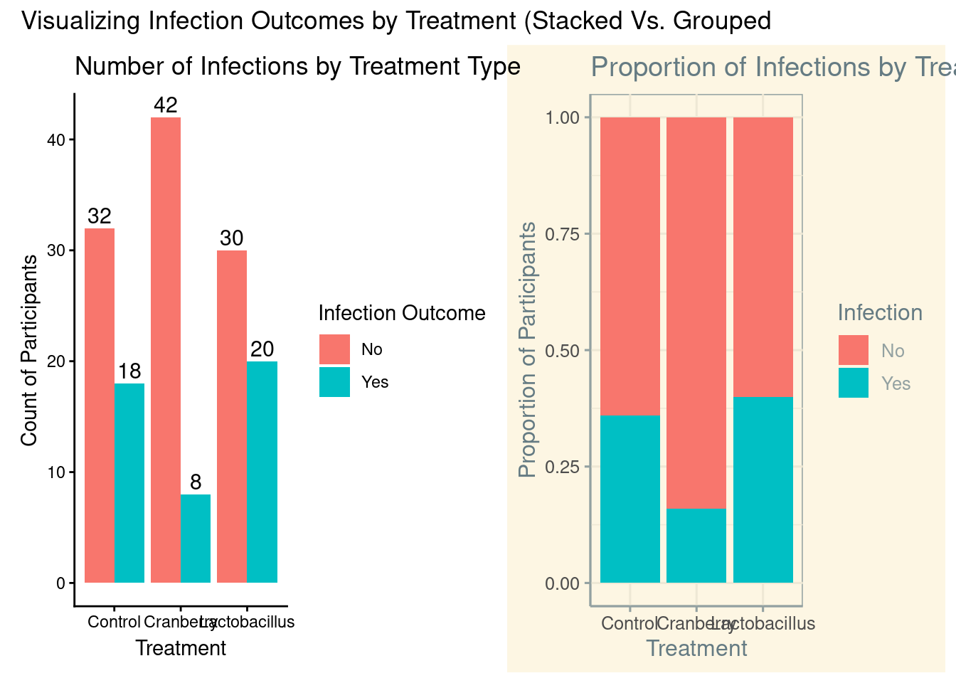
From a percentage standpoint, we see that 84% of people who were given cranberries were not infected! That is much higher than either other treatment options, and the total percentage of people who were not infected as well.
It seems that cranberry is taking an early lead in terms of which treatment is the most impactful. We have some preliminary numbers, so now we can visualize.
6.5 Visualizations
With purely categorical data, the visualization most commonly recommended would be a bar chart. With a bar chart, a viewer can interpret differences between the variables. There are two main options, a stacked or grouped bar chart. The main difference from a coding perspective is what we enter inside the geom_bar command.
# We can use the library ggthemes to add some flavor to our plotslibrary(ggthemes)# Creating a stacked bar chartstacked <-ggplot(infection, aes(x = Treatment, fill = Infection)) +geom_bar(position ="fill") +# "fill" stacks to 100% heightlabs(title ="Proportion of Infections by Treatment Type",y ="Proportion of Participants",x ="Treatment" ) +theme_solarized()
# Creating a grouped bar chartgrouped <-ggplot(infection, aes(x = Treatment, fill = Infection)) +geom_bar(position ="dodge") +geom_text(stat ="count", # use counts from geom_baraes(label =after_stat(count)), # label each bar with its countposition =position_dodge(width =0.9), # place correctly over side-by-side barsvjust =-0.3, # move labels slightly above barssize =4 ) +labs(title ="Number of Infections by Treatment Type",x ="Treatment",y ="Count of Participants",fill ="Infection Outcome" ) +theme_classic()
# We can put them side by side to compare what they look likelibrary(patchwork)grouped + stacked +plot_annotation(title ="Visualizing Infection Outcomes by Treatment (Stacked Vs. Grouped")
Figure 6.1: Side-by-side comparison of stacked and grouped bar charts visualizing infection outcomes by treatment type. The stacked chart emphasizes proportional differences, while the grouped chart highlights raw counts. Together, these plots illustrate how different visual encodings can influence interpretation of categorical data.
To make our graphs more interactive with our users, we can utilize the ggplotly() function from the plotly package.
# We can also use the plotly package to make the visual more interactivelibrary(plotly)ggplotly(grouped)
Figure 6.2: Interactive grouped bar chart displaying counts of infection outcomes by treatment type. Interactivity allows users to hover over bars to inspect values directly, supporting exploratory analysis while preserving the same information shown in the static grouped bar chart.
NoteWhen using ggplotly:
Move your cursor over the bars to gather more insights about your graph/data.
6.6 Chi-Square Test
Now, we have done some investigation on our data through contingency tables and visualizations. It is time to run what is called a chi-square test. This allows us to see if two categorical variables are related to each other.
Table 6.7: Chi-Square Test of Independence: Assessing the Relationship between Treatment Group and Infection Status.
Whether we performed it on our contingency table, we get:
X^2- This is the test statistic. This is telling us how much different our observed is vs our expected.
df - Degrees of freedom = (rows - 1)(columns - 1). For 3 treatments and 2 outcomes, df = (3-1)(2-1) = 2.
p-value- This tells us if it is statistically significant or not.
We see that our X^2 value is 7.78, our df is 2, and our p-value is 0.0204871. Since our p-value is less than .05, we can rightly say that there is a significant relationship between treatment plans and outcomes.
Now that we know it is significant, we need to dive a little deeper. We are understanding that cranberry is looking like the leader, but we can become more solidified on that stance.
chi_square_test <-chisq.test(contingency_table)# All the parts of the chi square can be called.chi_square_test$statistic
X-squared
  7.77592
chi_square_test$parameter
df
 2
chi_square_test$p.value
[1] 0.0204871
chi_square_test$method
[1] "Pearson's Chi-squared test"
chi_square_test$data.name
[1] "contingency_table"
# What our data already ischi_square_test$observed
               Infection
Treatment       No Yes
  Control       32  18
  Cranberry     42   8
  Lactobacillus 30  20
# What our data would look like if there was no relationshipchi_square_test$expected
               Infection
Treatment             No      Yes
  Control       34.66667 15.33333
  Cranberry     34.66667 15.33333
  Lactobacillus 34.66667 15.33333
# Difference between observed and expected# Positive is more than expected# Negative is less than expected# Bigger number = bigger difference# Represent how many standard deviationschi_square_test$residuals
               Infection
Treatment               No        Yes
  Control       -0.4529108  0.6810052
  Cranberry      1.2455047 -1.8727644
  Lactobacillus -0.7925939  1.1917591
# Standard Residuals# More like an actual z-scorechi_square_test$stdres
               Infection
Treatment              No       Yes
  Control       -1.001671  1.001671
  Cranberry      2.754595 -2.754595
  Lactobacillus -1.752924  1.752924
TipRule of Thumb:
Think of standardized residuals like z-scores: values greater than +2 or less than -2 are the ‘statistically interesting’ parts of your table that are driving your p-value.
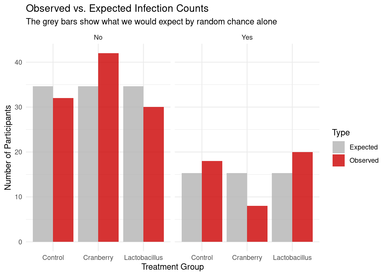
We can also visualize our observed versus our expected counts, as visualizations are key to understanding our data.
# 1. Extract observed and expected counts from our test objectobs_exp_data <-data.frame(Treatment =rep(rownames(chi_square_test$observed), 2),Infection =rep(colnames(chi_square_test$observed), each =3),Observed =as.vector(chi_square_test$observed),Expected =as.vector(chi_square_test$expected))# 2. Pivot the data to a 'long' format for ggplotplot_data <- obs_exp_data %>%pivot_longer(cols =c(Observed, Expected), names_to ="Type", values_to ="Counts")# 3. Create the plotggplot(plot_data, aes(x = Treatment, y = Counts, fill = Type)) +geom_bar(stat ="identity", position ="dodge", alpha =0.8) +facet_wrap(~Infection) +scale_fill_manual(values =c("Expected"="grey70", "Observed"="#CC0000")) +labs(title ="Observed vs. Expected Infection Counts",subtitle ="The grey bars show what we would expect by random chance alone",x ="Treatment Group",y ="Number of Participants" ) +theme_minimal()
Figure 6.3: Comparison of Observed vs. Expected counts across treatment groups. The ‘Expected’ bars represent the distribution of infections if the null hypothesis were true (no relationship). The visible gap between the observed and expected bars in the Cranberry group illustrates the ‘surprise’ in the data that drives the significant Chi-Square result.
Our deep dive uncovered some very important things about our experiment:
Expected: all of the values were different from what we the actual observations were. If there was no relationship between the two variables, it was expected that each treatment would have about 35 people not infected, and 15 people infected
Residuals/stdres: this is where we really start to tie everything together. With the residuals, we are looking for if it is positive/negative, and then strength in relation to the other. Cranberry if the only one of the three where there are less people infected than anticipated, almost 2 standard deviations less than expected. Both other treatments have more people infected than expected.
Note: Standardized residuals behave like z-scores — values beyond ±2 suggest cells contributing most strongly to the overall χ² statistic.
We tie this information together to get a very strong case for cranberry. There is just one piece of the puzzle left to bring this home.
6.7 Cross Tables
In the gmodels package we are able to utilize the CrossTable command. Beware, this can at first be overwhelming, as a lot of information is thrown at you.
Table 6.8: Comprehensive Cross-Tabulation: Observed and Expected Frequencies, Row/Column Proportions, and Chi-Square Contributions by Treatment and Infection Status.
library(gmodels)
Warning: package 'gmodels' was built under R version 4.5.2
# This allows us to see the contributions each category has on chi-square.# Note, you (infection$Treatment, infection$Infection) if you want to stick to defaultsCrossTable(infection$Treatment, infection$Infection,prop.chisq =TRUE, # Shows the chi-square contributionchisq =TRUE, # shows chi-square testexpected =TRUE, # shows expected countsprop.r =TRUE, # shows row proportionsprop.c =TRUE) # shows column proportions
CrossTable gave us a lot of information (nothing we can not handle). Thankfully, there is an legend in the beginning of the results that identifies what each number is. Some of these we already discovered, such as expected values and the chi-square X^2 value, but also some new information. Specifically, we are able to see the chi-square contribution. To break this down:
When we run the chi-square test, we get the X^2 value. Importantly, each combination of the variables contributes individually to this number. We are looking for the biggest contributors to not only understand the chi-square value better, but to also understand what is the most impactful.
For this result, our third number’s in each cell are the chi-square contribution. It is evident that cranberry has the highest contribution to the chi-square test statistic.
6.8 Contribution
If we want to hone in on this more, we can take the contributions and turn them into percentages.
TipTo find out more about the X^2 value, it is important to answer the question:
What percentage of the X^2 value is each contribution responsible for?
Table 6.9: Cell-wise Contributions to the Chi-Square Statistic: Identifying Discrepancies Between Observed and Expected Frequencies.
# Calculate contribution to chi-square statisticcontributions <- ((chi_square_test$observed-chi_square_test$expected)^2)/chi_square_test$expectedcontributions
               Infection
Treatment              No       Yes
  Control       0.2051282 0.4637681
  Cranberry     1.5512821 3.5072464
  Lactobacillus 0.6282051 1.4202899
TipThe formula for calculating the chi-square statistic is:
\[X^2= ((observed-expected)^2)/expected\]
Table 6.10: Percentage of Total Chi-Square Variance by Cell: Quantifying the Relative Impact of Each Treatment on the Overall Significance.
               Infection
Treatment              No       Yes
  Control        2.637993  5.964158
  Cranberry     19.949821 45.103943
  Lactobacillus  8.078853 18.265233
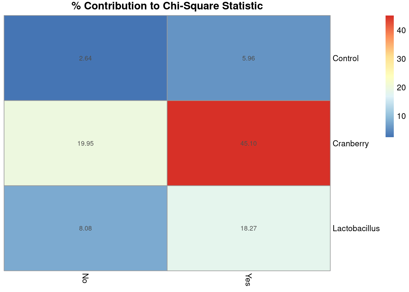
Through this, we discovered that about 65% of the X^2 value is due to the cranberry treatment.
You already know that visualizations really help paint the picture, and chi-square contributions are not exempt. For this, the pheatmap package comes in handy.
library(pheatmap)
Warning: package 'pheatmap' was built under R version 4.5.2
# Create heatmap for percentage contributionspheatmap(percent_contributions,display_numbers =TRUE,cluster_rows =FALSE,cluster_cols =FALSE,main ="% Contribution to Chi-Square Statistic")
Figure 6.4: Heatmap showing the percentage contribution of each cell to the overall chi-square statistic. Darker shading indicates cells that contribute more strongly to the chi-square value, highlighting which combinations of treatment type and infection outcome drive the observed association. This visualization helps identify where deviations from expected counts are largest following a significant chi-square test.
That glaring, deep red box? That is the cranberry yes cell!
Tying all of this together, we have discovered:
Cranberry has the most people that were not infected (least amount infected).
The chi-square test shows a significant relationship between treatment and outcome.
When looking at residuals, cranberry was the only treatment with less people infected than expected.
When looking at chi-square contributions,cranberry had the largest contribution, with about 65% of the test statistic being accounted for by cranberry.
Now, how impactful is this overall? What is the effect of treatment overall on outcome?
6.9 CramerV
Cramer’s V tells you the strength of the relationship between two categorical variables, similar to correlation coefficient It is important to note that this measures effect size. This is not a statistic. We can utilize the cramerV command from the rcompanion package.
library(rcompanion)cramerV(contingency_table)
Cramer V
  0.2277
The value derived from this is 0.23. Again, similar to the correlation coefficient, there are guidelines that can be utilized to understand the strength.
Table 6.11: Guidelines for interpreting the strength of association using Cramer’s *V*. These ranges provide general heuristics for describing effect size in categorical analyses and should be interpreted in context rather than as strict cutoffs.
Cramer V Value
Strength of Relationship
0.00–0.10
Very Weak
0.10–0.30
Weak
0.30–0.50
Moderate
>0.50
Strong
Treatment, overall, had a weak-moderate effect on outcome overall. This suggests that while treatment type and infection outcome are related, the relationship isn’t strong — meaning that other factors likely play a larger role.
6.10 Interpretation
The chi-square test shows X^2 = 7.78, df = 2, p = 0.02
This means there is a statistically significant relationship between Treatment and Infection.
The Cranberry group had fewer infections than expected and contributes most to the chi-square statistic.
Cramer’s V shows the relationship is weak-to-moderate in strength.
Drink your cranberry juice!
6.11 Key Takeaways
The Chi-Square test helps us determine whether two categorical variables are related.
It compares the observed frequencies (what we saw) to the expected frequencies (what we’d expect by chance).
A large Chi-Square statistic and a p-value < .05 suggest that the relationship is statistically significant.
Degrees of freedom (df) are based on the number of categories: (rows - 1) * (columns - 1).
Cramer’s V measures the strength of the relationship, similar to a correlation coefficient:
Residuals show which specific groups contribute most to the Chi-Square result.
Visualizations (like bar charts or heatmaps) make it easier to interpret where the differences lie.
Statistical significance ≠ practical significance — even weak relationships can be significant with large samples.
Example takeaway: Cranberry treatment showed fewer infections than expected — a weak but meaningful effect!
6.12 Checklist
When running a Chi-Square test, have you:
6.13 Key Functions & Commands
The following functions and commands are introduced or reinforced in this chapter to support categorical data analysis, contingency tables, and Chi-Square testing.
table()(base R)
Creates basic contingency (frequency) tables for categorical variables.
xtabs()(base R)
Constructs contingency tables using a formula interface, useful for multi-way tables.
tabyl()(janitor)
Generates clean contingency tables that integrate easily with percentage calculations.
adorn_percentages()(janitor)
Converts contingency table counts into row- or column-based percentages.
adorn_ns()(janitor)
Displays counts and percentages together for clearer interpretation.
chisq.test()(stats)
Performs a Chi-Square test of independence to assess whether two categorical variables are related.
CrossTable()(gmodels)
Produces detailed cross-tabulations including expected counts, proportions, and chi-square contributions.
pheatmap()(pheatmap)
Visualizes Chi-Square contributions or residuals using a heatmap.
cramerV()(rcompanion)
Computes Cramer’s V to measure the strength of association between categorical variables.
6.14 Example APA-style Write-up
The following example demonstrates one acceptable way to report the results of a chi-square test of independence in APA style.
Chi-Square Test of Independence
A chi-square test of independence indicated a significant association between treatment type and infection outcome, \(\chi^2(2, N = 150) = 7.78, p = .02\). The strength of this association was weak-to-moderate, Cramer’s \(V = .23\). As illustrated in Figure 6.4, the primary driver of this significance was the Cranberry group, which exhibited fewer infections than would be expected by chance.
6.15 💡 Reproducibility Tip:
It is essential to both visually and structurally inspect your data, because data are not always what they seem.
Consider Advanced Placement (AP) exam scores in U.S. high schools. Students receive scores from 1 to 5. While these values look numeric, they are actually categorical—there is no meaningful value like 2.5. Treating them as numeric can lead to incorrect analyses. The same issue commonly arises with variables like zip codes, which may be stored as numbers but represent categories, not quantities.
Although functions like View() or head() are useful for visually checking your data, they do not reveal how R is interpreting each variable. Always use functions like str() to confirm that variables are stored with the correct data type before running an analysis.
Analyses based on incorrectly typed variables are not reproducible—because they are not valid to begin with.